Building Placement: Reinforcement Learning
In the previous section, we demonstrated that our building placement model works well in a supervised setup. Here, we'll discuss how to learn placement in a reinforcement learning (RL) setting. We assume familiarity with common RL concepts that can, if necessary, be acquired through various online classes. Prominent examples are David Silver's course at UCL or the Deep Reinforcement Learning course at Berekely.
Action Space Restriction by Masking
As discussed in the Neural Network Architecture section, the model outputs a probability distribution for every possible build location on the entire map. In an RL setup, this results in 128x128 = 16384 actions, many of which are impossible to perform due to limited terrain buildability or game constraints (e.g. most Zerg structures can only placed on creep). Furthermore, we formulated the building placement problem as to be restricted to a target BWEM area in the introduction.
In order to speed up learning, we want to avoid needless exploration and will thus restrict the action space of the model to the valid placement positions at the time when the placement action is taken. A location is considered valid if
- It is within the target BWEM area
- It is on buildable terrain
- If a couple of hard-coded placement checks are successful. These account for the size of the building to be placed and positions of other buildings that have been placed but for which construction has not been started, for example.
For the supervised training setup, we provided the model with an input that marked the target area. However, learning the mapping from multiple inputs to valid and invalid actions is time-consuming in reinforcement learning. We thus opt for masking out invalid actions instead, so that the probabilities computed by the model will be non-zero for valid locations only. This is achieved by applying a mask \(m\) of valid actions (i.e. with values 1 for valid and 0 for invalid actions) during the softmax computation as follows: $$\operatorname{masked\_softmax}({\bf x}, {\bf m})_i = \frac{m_i e^{x_i}}{\sum_i m_i e^{x_i}}$$
In the scenario we consider below, this reduces the action space from 16384 to 10 to 50, depending on the respective game state. In fact, in some cases we will consider only a single valid action and bypass the model completely: placing extractors and expansions.
Example Scenario
In the example scenario we consider, expansion placement is crucial for winning the game. Both players play Zerg and are implemented with TorchCraftAI. The opponent quickly builds up pressure by producing Zerglings, while the player that we're considering for learning tries to transition to Mutalisks. If it succeeds, it has a significant edge over the opponent, which cannot defend against air attacks. However, the technology investment requires withstanding the Zergling pressure by placing Sunken Colonies for defense. If those are purely placed, our player gets defeated quickly.
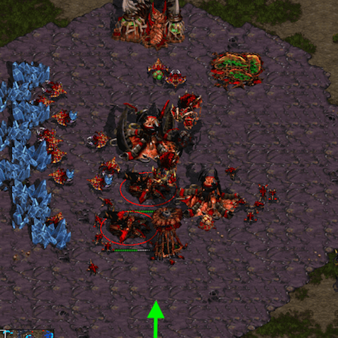
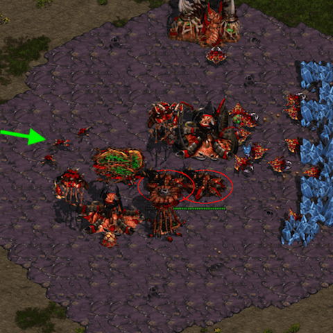
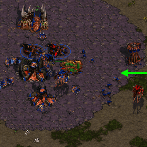
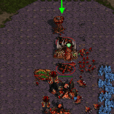
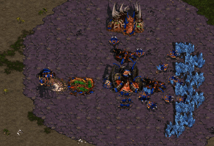
Check out two sample replays for a game we win and a game we lose with the built-in placement rules. In both replays, "BWEnv1_Zerg" is the player placing the defense buildings. The resulting building layout looks like this, and its effectiveness in withstanding the Zergling attack (of our built-in rules) is largely determined by the direction by which enemy units approach the base.
Training Program
From a high-level perspective, our training setup and code follows the training blueprint for a high-level model since we're not interested micro-control of individual units but rather take a macro-action that will be carried out by the rule-based BuilderModule. We'll discuss the individual files in the tutorial folder (tutorials/building-placer) below.
RLBuildingPlacerModule
The module implementation in rlbuildingplacer.cpp closely follows the stock BuildingPlacer module but contains additional logic and book-keeping to enable RL training.
RLBuildingPlacer::upcWithPositionForBuilding() contains the code that executes Trainer::forward() and translates the action sampled from the model output to a UPCTuple.
Specifically, it
- uses the built-in placement rules to obtain a seed position. This position determines the BWEM area we'll pass to the model
- falls back to the seed position for actions we don't want to let the model take, e.g. placing expansions
- constructs a
BuildingPlacerSampleobject from the current game state - calls
Trainer::forward() - constructs a
RLBPUpcDatainstance containing the sample and the model output. TheRLBPUpcDatainstance will then be posted to the Blackboard alongside the UPCTuple as discussed in the training blueprint.
The module also implements a custom proxy task to react to cancellations and to detect whether a building has been started.
One implementation detail of the rule-based TorchCraftAI modules is that the build order will cancel the building creation task as soon as the building appears in the game state.
Hence, extra tracking for successful building creation is performed in RLBuildingPlacerModule::step():
  // Check ongoing constructions
  auto constructions = state->board()->get(
      kOngoingConstructionsKey, std::unordered_map<int, int>());
  for (auto& entry : constructions) {
    auto upcId = entry.first;
    auto* unit = state->unitsInfo().getUnit(entry.second);
    if (unit->completed()) {
      markConstructionFinished(state, upcId);
    } else if (unit->dead) {
      markConstructionFailed(state, upcId);
    }
  }
Finally, the trainer frames for each action \( a_t \) are submitted in onGameEnd() using the following reward scheme:
$$
\begin{equation}
R(a_t) =
\begin{cases}
+0.5 ,& \text{building for $a_t$ was started and the game was won} \\
-0.5 ,& \text{building for $a_t$ was started and the game was list} \\
0,& \text{otherwise} \\
\end{cases}
\end{equation}
$$
Main Loop
The main training loop is implemented in train-rl.cpp and can perform both RL training and evaluation of either trained models or the built-in rules. The training can either be run for a maximum number of updates or a maximum number of training games.
During training, intermediate models are regularly evaluated; by default, this happens after 500 model updates.
The evaluation frequency can be adjusted with the -evaluate_every command-line flag.
Code-wise, training and evaluation work similarly.
We create a cpid::Evaluator with a sampler that always takes the action with the maximum probability and plays a fixed number of games.
void runEvaluation(
    std::shared_ptr<Trainer> trainer,
    int numGames,
    std::shared_ptr<MetricsContext> metrics) {
  int gamesPerWorker = numGames / dist::globalContext()->size;
  int remainder = numGames % dist::globalContext()->size;
  if (dist::globalContext()->rank < remainder) {
    gamesPerWorker++;
  }

  trainer->model()->eval();
  auto evaluator = trainer->makeEvaluator(
      gamesPerWorker, std::make_unique<DiscreteMaxSampler>("output"));
  evaluator->setMetricsContext(metrics);
  metrics->setCounter("timeout", 0);
  metrics->setCounter("wins_p1", 0);
  metrics->setCounter("wins_p2", 0);

  // Launch environments. The main thread just waits until everything is done
  std::vector<std::thread> threads;
  for (auto i = 0; i < FLAGS_num_game_threads; i++) {
    threads.emplace_back(runGameThread, evaluator, i);
  }

  while (!evaluator->update()) {
    std::this_thread::sleep_for(std::chrono::milliseconds(100));
  }

  evaluator->setDone();
  evaluator->reset();
  for (auto& thread : threads) {
    thread.join();
  }

  // Sync relevant metrics
  static float mvec[3];
  mvec[0] = metrics->getCounter("games_played");
  mvec[1] = metrics->getCounter("wins_p1");
  mvec[2] = metrics->getCounter("wins_p2");
  dist::allreduce(mvec, 3);
  metrics->setCounter("total_games_played", mvec[0]);
  metrics->setCounter("total_wins_p1", mvec[1]);
  metrics->setCounter("total_wins_p2", mvec[2]);

  trainer->model()->train();
}

void trainLoop(
    std::shared_ptr<Trainer> trainer,
    std::shared_ptr<visdom::Visdom> vs) {
  // ...

  auto evaluate = [&]() -> float {
    gResultsDir = fmt::format("eval-{:05d}", numModelUpdates);
    fsutils::mkdir(gResultsDir);

    auto evalMetrics = std::make_shared<MetricsContext>();
    runEvaluation(trainer, FLAGS_num_eval_games, evalMetrics);
    evalMetrics->dumpJson(
        fmt::format(
            "{}/{}-metrics.json", gResultsDir, dist::globalContext()->rank));
    auto total = evalMetrics->getCounter("total_games_played");
    auto winsP1 = evalMetrics->getCounter("total_wins_p1");
    return float(winsP1) / total;
  };

  // ...
}
Scenario
The scenario we'll consider is defined in scenarios.cpp and set up with a provider called SunkenPlacementScenairoProvider.
For each game, a map from a pre-defined map pool will be selected at random, and players will be set up to play custom buildorders defined in tutorials/building-placer/buildoders.
The players returned from from spawnNextScenario() are ready to be used for playing a game.
class SunkenPlacementScenarioProvider : public BuildingPlacerScenarioProvider {
 public:
  SunkenPlacementScenarioProvider(std::string mapPool, bool gui = false)
      : BuildingPlacerScenarioProvider(kMaxFrames, std::move(mapPool), gui) {}

  virtual std::pair<std::shared_ptr<BasePlayer>, std::shared_ptr<BasePlayer>>
  spawnNextScenario(
      const std::function<void(BasePlayer*)>& setup1,
      const std::function<void(BasePlayer*)>& setup2) override {
    map_ = selectMap(mapPool_);
    loadMap<Player>(
        map_,
        tc::BW::Race::Zerg,
        tc::BW::Race::Zerg,
        GameType::Melee,
        replayPath_);

    setupLearningPlayer(player1_.get());
    setupRuleBasedPlayer(player2_.get());

    // Set a fixed build for both players
    build1_ = "9poolspeedlingmutacustom";
    build2_ = "10hatchlingcustom";
    player1_->state()->board()->post(Blackboard::kBuildOrderKey, build1_);
    player2_->state()->board()->post(Blackboard::kBuildOrderKey, build2_);

    // Finish with custom setup
    setup1(player1_.get());
    setup2(player2_.get());

    std::static_pointer_cast<Player>(player1_)->init();
    std::static_pointer_cast<Player>(player2_)->init();
    return std::make_pair(player1_, player2_);
  }
};
Custom Policy Gradient Trainer
In this tutorial, we opt for implementing a custom cpid::Trainer in bpgtrainer.h.
It is largely inspired by cpid::BatchedPGTrainer but differs in a few details:
For one, experience frames are sampled on a per-transition bases rather than on a per-episode basis.
This ensures equal mini-batch sizes across updates, which in turns stabilizes learning.
The trainer also adds an entropy regularization term to the standard REINFORCE criterion in order to encourage exploration by smoothing the model output The scaling factor of the entropy term takes the varying action space between model decisions into account (which originates from state-dependent masking as discussed above) and is defined on the model output \(o\) and mask \(m\) as $$ L_E({\bf o}, {\bf m}) = \frac{1}{\eta * \ln \left( \sum_i m_i - 1 \right)} \sum_i o_i \ln o_i $$ \( \eta \) is hyper-parameter to scale the general influence of the entropy loss and hence defines the peakiness of the model output distribution.
Last but not least, support for value functions was removed as we did not find it helpful for the specific setup discussed here.
Training and Evaluation
The training can be run by starting ./build/tutorials/building-placer/bp-train-rl.
The program povides many options (see the start of train-rl.cpp or, for a full list of command-line flags, pass -help), but the default settings produced stable learning in our runs.
For less verbose output from the main bot code, run the program as
./build/tutorials/building-placer/bp-train-rl -v -1 -vmodule train-rl=1.
Note that in order to run distributed (multi-machine) training, additional arguments are required:
-c10d_size Nto specify the total number of processes-c10d_rank Ito specify the rank of each process that is started-c10d_rdvu file:LOCATIONto perform the initial process rendez-vous using the file path LOCATION. This path must be accessible from all processes, i.e. reside on a shared file system. Each of our training jobs ran on 8 machines, using 40 CPU cores and 1 GPU on each host, but we've seen resonable learning progress with fewer machines as well.
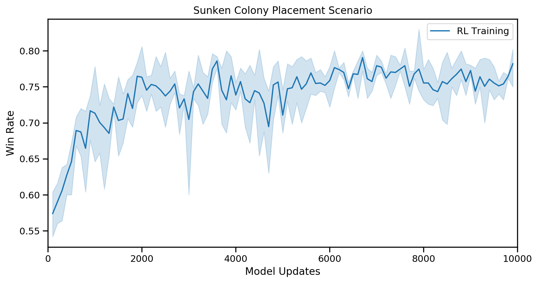
Over 10,000 updates, intermediate win rate evaluations produced the following graphs across 3 different runs:
How does this compare to the default placement rules? To obtain final numbers, let's run a larger evaluation with the default rules and the final models obtained by reinforcement learning, e.g. after 10000 updates using the checkpoint:
./build/tutorials/building-placer/bp-train-rl -evaluate rules -num_eval_games 5000
#
# ... after quite a lot of output, and possibly quite some time:
#
I81060/XXXXX [train-rl.cpp:749] Done! Win rates for 5000 games: 65.8% 34.2%

./build/tutorials/building-placer/train-rl -evaluate argmax -num_eval_games 5000 -checkpoint /path/to/final/checkpoint
#
# ...
#
I30983/XXXXX [train-rl.cpp:749] Done! Win rates for 5000 games: 78.5% 21.5%
The rules have an average win rate of 65.8% while an RL-trained model achieves 78.5% -- an improvement of over 10% absolute. The final win rates of our trained models vary a bit from run to run but final results should be in the mid-70s.
Let's look at the layout that the model produces for the different starting positions on Fighting Spirit. For illustration purposes, the direction in which enemy units have to take to enter the main base via the ramp is indicated with a green arrow. Click on the images to download the respective replays.
The two highlighted Sunken Colonies are placed very differently for each spawning position of the map and roughly correspond to the angle of the early Zergling atttack. A notable observation is that in the lower right, the Spire is exposed as it was placed outside of the Sunken range. This is an artifact of playing against the built-in rules: the attacker will simply ignore the Spire and rush straight into the base.

